Let’s demo RivGraph on the Brahmaputra River!
This demo shows some of the core functionality and convenient plotting and exporting features provided by RivGraph for a braided river network. The basic steps of RivGraph-ing a braided river include:
Instantiate river class
Skeletonize the binary mask
Compute the network (links and nodes)
Prune the network
Compute morphologic metrics (lengths, widths)
Compute a mesh (6.1 - Adjust mesh parameters)
Assign flow directions for each link
A note on topologic metrics
Along the way, we’ll export some geotiffs and GeoJSONs (or shapefiles if you prefer) for inspection in QGIS. RivGraph requires a binary mask of the channel network, preferably georeferenced (i.e., a GeoTiff) in a projected coordinate reference system.
1. Instantiate river class
from rivgraph.classes import river
import matplotlib.pyplot as plt
import os

# Define the path to the georeferenced binary image.
mask_path = './data/Brahmaputra_Braided_River/Brahmaputra_mask.tif'

# Results will be saved with this name
name = 'Brahma'

# Where to store RivGraph-generated geotiff and geovector files.
results_folder = './data/Brahmaputra_Braided_River/Results'

# Set the exit sides of the river relative to the image. In this case, the
# Brahmaputra is "entering" the image from the North and "exiting" the
# image from the South.
es = 'NS' # The first character is the upstream side

# Boot up the river class! We set verbose=True to see progress of processing.
brahma = river(name, mask_path, results_folder, exit_sides=es, verbose=True)

# The mask has been re-binarized and stored as an attribute of brahma:
plt.imshow(brahma.Imask)
<matplotlib.image.AxesImage at 0x1eb4f279e50>
2. Skeletonize the binary mask
# Simply use the skeletonize() method.
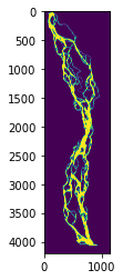
brahma.skeletonize()
# The skeletonized image is stored as an attribute to the brahm class. Let's take a look.
plt.imshow(brahma.Iskel)
<matplotlib.image.AxesImage at 0x1eb4f7e90a0>
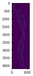
The skeleton is hard to see; perhaps we’d like to look at it closer? One option is to save it as a geotiff and pull it up in a GIS (like QGIS).
# We use the write_geotiff() method with the 'skeleton' option.
brahma.to_geotiff('skeleton')
Geotiff written to dataBrahmaputra_Braided_RiverResultsBrahma_skel.tif.
The georeferenced Brahmaputra skeleton has been written to disk, so we can pull it up in QGIS along with the georeferenced mask:
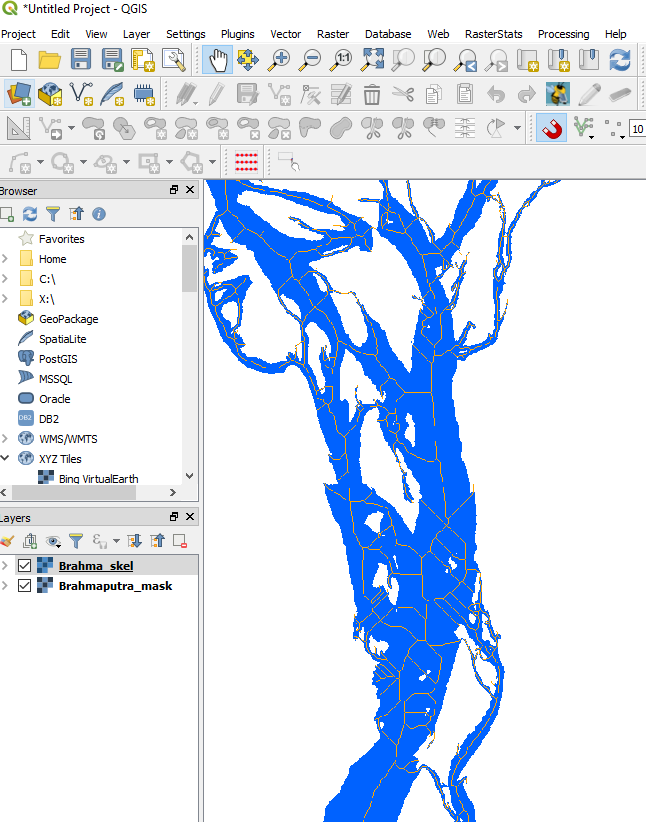
brahma_qgis_mask_skel.PNG
3. Compute the network (links and nodes)
# Simply use the compute_network() method.
brahma.compute_network()
Resolving links and nodes...done.
# Now we can see that the "links" and "nodes" dictionaries ahve been added
# as attributes to the brahma class:
links = brahma.links
nodes = brahma.nodes
print('links: {}'.format(links.keys()))
print('nodes: {}'.format(nodes.keys()))
links: dict_keys(['idx', 'conn', 'id', 'n_networks'])
nodes: dict_keys(['idx', 'conn', 'id'])
The links dictionary currently contains four keys: - idx: a list of all the pixel indices that make up the link (indices created with input mask shape and np.ravel_multi_index) - conn : a two-element list containing the node ids of the link’s endpoints - id: each link has a unique id; the ordering is irrelevant - n_networks: the number of disconnected networks (==1 if the input mask contains a single connected blob)
The nodes dictionary currently contains three keys: - idx: the index of the node’s position within the original image (i.e. np.ravel_multi_index()) - conn: an N-element list containing the N link ids of the links connected to this node. - id: each node has a unique id; the ordering is irrelevant
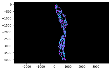
We can visualze the network in a couple of ways. First, we can plot with matplotlib:
brahma.plot('network')
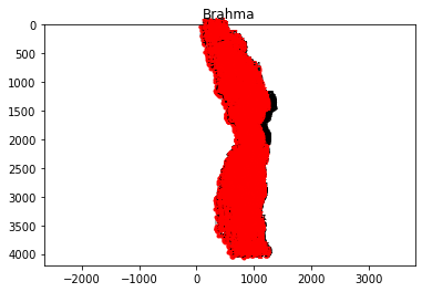
Nodes and links are labeled with their ids. We can zoom in if plotting in an interactive matplotlib window, or we can export the network links and nodes as geovector files and pull ’em into QGIS:
brahma.to_geovectors('network', ftype='json')

# Let's see where the network geovector files were written:
print(brahma.paths['links'])
print(brahma.paths['nodes'])
dataBrahmaputra_Braided_RiverResultsBrahma_links.json
dataBrahmaputra_Braided_RiverResultsBrahma_nodes.json
And dragging these into QGIS: 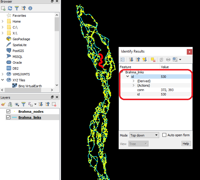 You can
query different links and nodes using the Identify tool. Note that their
properties (‘conn’ and ‘id’) are appended.
You can
query different links and nodes using the Identify tool. Note that their
properties (‘conn’ and ‘id’) are appended.
If you pan around a bit, you’ll notice that there are many “dangling” links, or links connected only at one end. These links play no role in the connectivity of the network, and we therefore may want to remove them. We don’t want to remove the inlet and outlet links, however. RivGraph will prune these dangling links but preserve the inlet and outlet links by exploiting the exit_sides we supplied earlier. Let’s prune the network.
4. Prune the network
brahma.prune_network()

# We see that 'inlets' and 'outlets' have been added to the nodes dictionary:
print(brahma.nodes.keys())

# We can get the node ids of the inlets and outlets
print('inlets:', brahma.nodes['inlets'])
print('outlets:', brahma.nodes['outlets'])
dict_keys(['idx', 'conn', 'id', 'inlets', 'outlets'])
inlets: [247]
outlets: [1919]
5. Compute morphologic metrics (lengths, widths)
Now that the network is resolved and pruned, we can compute some link metrics.
brahma.compute_link_width_and_length()

# Let's look at histograms of link widths and lengths:
trash = plt.hist(brahma.links['len_adj'], bins=50)
plt.ylabel('count')
plt.xlabel('link length (m)')
plt.title('Histogram of link lengths')
Computing distance transform...done.
Computing link widths and lengths...done.
Text(0.5, 1.0, 'Histogram of link lengths')
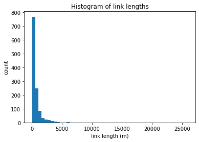
In the above figure, we see that almost all the links are shorter than 5 km. This histogram will be different for each braided river, and can depend on the resolution of your input binary mask. Resolving smaller channels generally, though not always, produces smaller average link lengths as longer links are broken to connect to the smaller ones.
Note: the lengths are reported in meters bcause that is the unit of the provided mask’s CRS (coordinate reference system). You can check this unit:
print(brahma.unit)
meter
6. Compute a mesh
In preparation for setting flow directions of each link, we will compute an “along-valley” mesh. This mesh is created based on the overall morphology of the braided river as opposed to individual channels within the network. The objective of the mesh is to create an along-channel grid that contains transects that are roughly perpendicular to the river “centerline” and approximately evenly-spaced.
While this mesh is necessary for setting flow directions, it is also useful for measuring along-river characteristics (like width, erosion rates, braiding index, etc.). The generation of this mesh requires a few parameters that ideally would be user-defined each time. However, for simplicity, RivGraph will make estimates of these parameters based primarily off the average link width. These parameters are described after we generate a default mesh.
# Note that we provide no arguments to the compute_mesh() function.
brahma.compute_mesh()
Computing centerline...done.
Computing link widths and lengths...done.
Generating mesh...done.
Before we play with the mesh-generation parameters, let’s take a look at
what we’ve generated with the compute_mesh() function.
First, we see that a centerline was computed. We can access this centerline:
print(brahma.centerline)
(array([764625., 764595., 764565., ..., 785475., 785505., 785535.]), array([2753535., 2753505., 2753475., ..., 2633625., 2633655., 2633655.]))
We get a numpy array of two arrays of columns, rows of the centerline. This isn’t very interpretable as-is, but we can export the centerline as a geovector file:
brahma.to_geovectors('centerline', ftype='json')
The centerline is exported as a shapefile or GeoJSON, depending on the filetype you specify. (GeoJSON is default.) Let’s take a look at this centerline in QGIS:
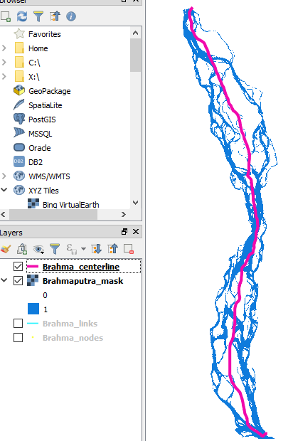
brahma_qgis_centerline.png
A little jagged, but it’s fine for our purposes. The centerline is computed by filling in all the islands of the network, then using a distance transform to find the “centermost” pixels.
Now let’s take a look at the mesh we generated. We first need to export it:
brahma.to_geovectors('mesh', ftype='json')
The mesh consists of two files: meshlines, or transects, and
meshpolys. If we want to see where these files were generated, we
can check the paths dictionary:
print(brahma.paths['meshlines'])
print(brahma.paths['meshpolys'])
dataBrahmaputra_Braided_RiverResultsBrahma_meshlines.json
dataBrahmaputra_Braided_RiverResultsBrahma_meshpolys.json
Let’s see what the mesh looks like by dragging these GeoJSONs into QGIS:
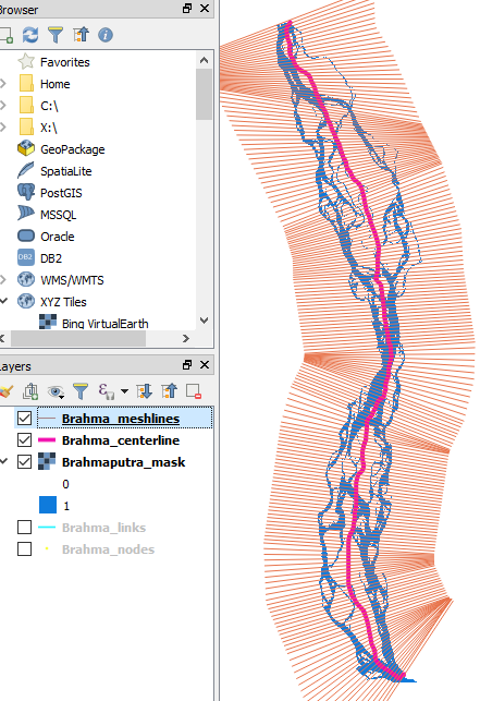
brahma_qgis_initial_meshlines.png
The mesh does a pretty good job of meeting our two criteria: approximately perpendicular to the centerline, and evenly-spaced along the centerline. It’s not perfect, but we can play with the parameters to adjust it.
6.1 Adjust mesh parameters
We may want to alter certain features of the mesh, like the spacing of
transects or the overall width of the mesh. When we call
compute_mesh(), there are three optional keyword arguments we can
provide to control mesh properties. These are:
grid_spacing : The along-centerline distance between each transect.
The default value is the average link width, found by
np.mean(brahm.links['wid_adj']).
smoothing : The degree of smoothing to perform on the centerline
before creating its offsets. This parameter is expressed in terms of the
fraction of the total centerline length, so the default
smoothing=0.1 will use a moving-average with a window size of 10% of
the length of the centerline.
buf_halfwidth : The distance from the centerline to each edgeline of
the buffer. The default is 10% wider than the maximum width of the mask,
which ensures that the mask is fully covered by the mesh.
We can check what values of each of these were used above:
# grid_spacing
print('grid_spacing: {}'.format(brahma.avg_chan_width))
# buf_halfwidth
print('buf_halfwidth: {}'.format(brahma.max_valley_width_pixels * brahma.pixlen * 1.1))
# smoothing by default was 0.1
print('smoothing: {}'.format(0.1))
grid_spacing: 623.1819853141467
buf_halfwidth: 15631.83213830036
smoothing: 0.1
You may have noticed that the mesh transects near the beginning of the reach (top of image) aren’t quite a perpendicular to the centerline as we might like. Let’s try smoothing the centerline a bit more and reducing the buffer width to make these more perpendicular. The grid spacing will not affect the overall mesh strucutre, so we’ll leave it the same for comparison purposes.
brahma.compute_mesh(buf_halfwidth=10000, smoothing=0.25)
Generating mesh...done.
Here’s a side-by-side comparison with the default mesh:
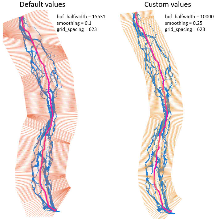
brahma_mesh_comparison.png
There are two primary differences between our custom mesh and the
default one. First, the custom mesh is narrower as a direct result of us
reducing buf_halfwidth from 15631 to 10000. Secondly, the custom
mesh transects are significantly more parallel to the centerline than
the default mesh. This resulted from increasing smoothing from 0.1
to 0.25. These two parameters, plus grid_spacing, can be used to
design a mesh to suit your needs.
7. Assign flow directions to each link
Now we want to determine the long-term, steady-state flow direction in each link. The algorithms used here are described in this paper.
brahma.assign_flow_directions()
Setting link directionality...Using dataBrahmaputra_Braided_RiverResultsBrahma_fixlinks.csv to manually set flow directions.
Attempting to fix 2 cycles.
All cycles were resolved.
done.
A statement appears that tells us that a .csv file was created for us to
set flow directions manually. This file is only created if it does not
already exist. So if we re-run assign_flow_directions(), we should
not see this message again.
brahma.assign_flow_directions()
Setting link directionality...Using dataBrahmaputra_Braided_RiverResultsBrahma_fixlinks.csv to manually set flow directions.
Attempting to fix 2 cycles.
All cycles were resolved.
done.
Now we see a message stating that RivGraph will use the .csv file to set flow directions manually. However, we haven’t populated the file yet so no there is no information for RivGraph to use. We’ll revisit this at the end of this section.
We also see a message stating that RivGraph is
Attempting to fix 2 cycles. A cycle is a set of links within a graph
that feeds into itself. RivGraph’s directionality algorithms enforce the
condition that no cycles should be present in the resulting graph. If
any cycles are found after setting all link directions, RivGraph
attempts to fix them. This does not mean that all the links’ directions
are correct, but rather that the resulting graph contains no cycles. In
this case, RivGraph was able to resolve both cycles.
Let’s inspect the resulting link directions. We again have two options: we can plot the links via matplotlib within Python:
brahma.plot('directions')
Cyan represents the upstream portion of a link, and magenta the downstream. As before, this is difficult to see without zoooming. So we can export a geotiff that contains directionality information for inspection in QGIS:
brahma.to_geotiff('directions')
Geotiff written to dataBrahmaputra_Braided_RiverResultsBrahma_link_directions.tif.
Dragging into QGIS (and adding a colorbar legend), we see
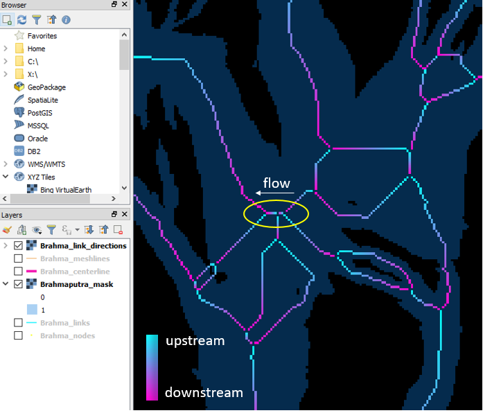
brahma_qgis_initial_directions.png
I’ve circled two short links in yellow, and noted that their flow direction was set as going right-to-left. Ideally, this junction would be comprised of a single node replacing these links, but RivGraph does not have the capability yet to simplify the network (a feature request has been made for this). From cursory inspection, we could make the argument that flow should instead go left-to-right for these two links. Let’s force flow the opposite direction as an example of how to manually set links.
First, we need to identify the link ID’s of each of these links, as well as the desired upstream nodes. Using the Identify tool in QGIS with the links and nodes GeoJSON layers turned on, this is easy:
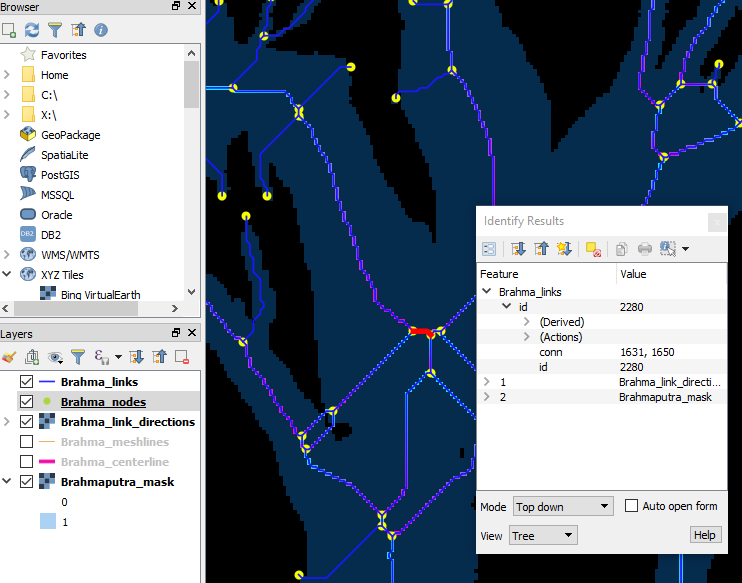
brahma_qgis_identify_links_for_reversal.png
We see that the red-highlighted link’s ID is 2280, and it’s
(upstream, downstream) nodes are 1631, 1650. We want to reverse this
order so that the upstream node ID is 1650. Open the
Brahma_fixlinks csv and enter this information. I have also done
this for the link to the right of this one.
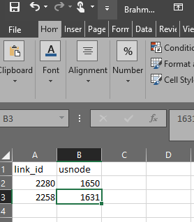
brahma_fixlinks_csv.png
Simply save the .csv and re-run the assign_flow_directions() method:
brahma.assign_flow_directions()
Setting link directionality...Using dataBrahmaputra_Braided_RiverResultsBrahma_fixlinks.csv to manually set flow directions.
Attempting to fix 2 cycles.
All cycles were resolved.
done.
After exporting the directions geotiff again, we can plot it against
the original:
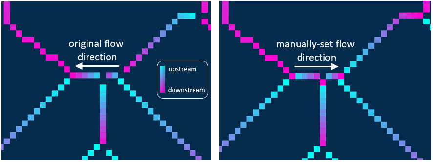
brahma_flow_direction_reversed_manually.png
We see that RivGraph used the information in our .csv to manually set the flow directions for both these links in the opposite direction of the original solution. It is important to note that RivGraph guarantees that whatever link flow directions are specified in the .csv will be preserved throughout the direction-setting process. RivGraph uses an iterative approach to set link directionalities, where knowing the direction of a nearby link can be used to set links of unknown directions. This means that if you incorrectly set a link’s direction manually, you could “infect” the nearby links with wrong directions! Indeed, we see from the above comparison that the upper-right link’s direction has also been reversed, even though we didn’t specify it. Whether or not this is correct is determined by the user.
8. A note on topologic metrics
If you’ve looked through the delta example, you’ll see the final section covers computing topolgic metrics. In order to compute these metrics, some additional finagling of the network is required. We have not yet implemented the required pre-processing for braided rivers. However, many of the functions in the delta metrics script can be used on braided rivers, provided you first pre-process your braided river network properly.