Maskmaking
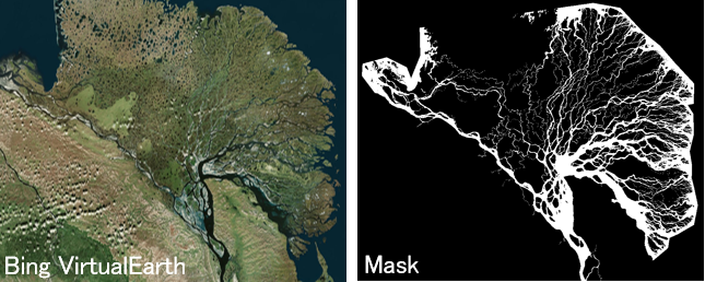
The Lena River Delta as seen by Bing Virtual Earth and its mask. Note that this mask is Landsat-derived so it does not correspond perfectly with the image on the left.
Maskmaker, Maskmaker Make Me a Mask
RivGraph requires that you provide a mask of your channel network. In this document, we’ll cover the following:
Important
One thing to keep in mind: although RivGraph contains functions for pruning and otherwise modifying your channel network, it will always honor the mask you provide. You may need to iterate between altering your mask and RivGraph-ing it to achieve your desired results. “Garbage in, garbage out.”
What is a mask?
A mask is simply a binary image (only ones and zeros) where pixels belonging to the channel network are ones, like the right panel of the Lena Delta above. Before processing your mask with RivGraph, you should ensure that your mask contains no no-data. One way to ensure this is to convert your mask to a boolean datatype, using for example numpy:
Mask_binary = np.array(Mask, dtype=np.bool)
The mask is the cornerstone for using RivGraph. You should always ensure that it contains the features you want and none of the ones you don’t.
Tip
Make sure to remove all the objects (connected “on” pixels) in your mask that you do not want to analyze. Leaving in other objects can cause unexpected behavior or errors. Often, a quick way to achieve this is via the rivgraph.im_utils.largest_blobs() function, which will keep only the largest connected component.
What does RivGraph expect my mask to look like?
RivGraph can handle two types of masks: deltas and braided (or single-threaded) rivers.
All masks should contain a single connected component (or blob). Before doing your analysis, use the rivgraph.im_utils.largest_blobs() to ensure you have only one connected component. This will remove any isolated portions of the mask. For example,
from rivgraph import im_utils
Mask_one_blob = im_utils.largest_blobs(Mask, nlargest=1, action='keep')
This will create an image wherein only the largest connected component remains (hopefully your channel network).
Delta masks often have a large waterbody (ocean or lake) connecting all the outlets. This is completely fine, as the waterbody will be removed in the pruning stage.
What should a mask capture?
Above, we defined a mask as all the pixels “belonging to the channel network.” But which pixels are part of the channel network? The obvious starting point is to consider all surface water pixels as defining the channel network. Is it important that your mask shows bankfull channels or includes small streams that may only be active during flood conditions?
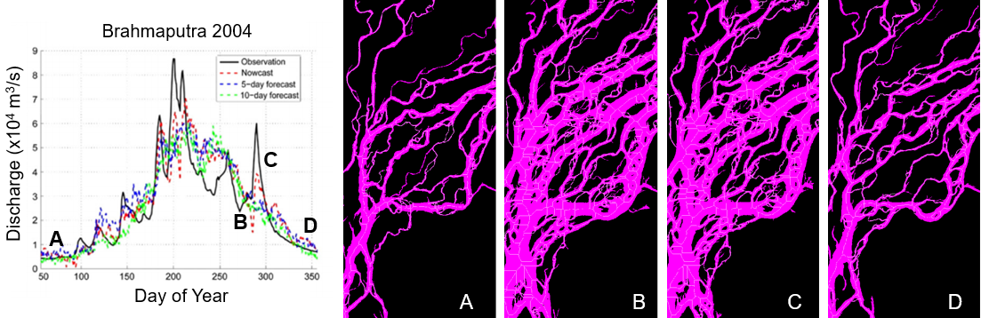
As an example, four masks are shown above of a portion of the Brahmaputra River at four different days of 2004. The hydrograph of the river is shown in the left panel. As expected, you can see that the mask changes as the river floods and recedes. You can also see that the river channel network has been rearranged in some places by the flooding. For example, A and D show the river at roughly the same discharge, but the network in D is a result of reworking by the flood.
The bottom line here is that your mask should reflect your analysis goals. For example, if you’re only interested in counting the number of loops in a delta channel network, then you might only care about ensuring all the channels are represented. If you want to route fluxes through your extracted network, then you probably should try to obtain a mask that captures the full width of the channels at some representative discharge.
Where do I get a mask?
Masks can come from a variety of sources, but in my experience there are three primary methods for mask generation:
automatically generated from satellite imagery
manually drawn by hand
model/simulation outputs
There are many methods available for creating masks automatically from remotely-sensed imagery. We won’t get into the details of those here, but note that machine learning has proved a very valuable tool for maskmaking. There are also simple, proven techniques available as well. The Brahmaputra masks above were created by thresholding the Landsat-derived NDVI (Normalized Difference Vegetation Index ), which is a simple ratio of band values.
Drawing a mask by hand is often not an ideal choice, but might be the most efficient way to move forward. In these cases, I would typically use QGIS to draw polygons that cover the channel network, then use the Rasterize tool to convert the polygons to a binary raster (image). If you go this route, be sure to specify an appropriate coordinate reference system for your polygons in order to preserve the georeferencing information (don’t use EPSG:4326). You will also need to specify a pixel resolution for your mask upon conversion.
If you’re analyzing the output of a simulation, it is unlikely that the simulation will provide binary channel masks as an output. In these cases, you will need to develop a way to identify the channel network from the available simulation results. For example, while developing the entropic Braided Index (eBI ), we used Delft3D simulations to test hypotheses about how the eBI changes under various sedimentation schemes. To make masks, we developed a combined depth + discharge threshold to identify which pixels were part of the “active river channel.”
Here are some resources that either provide masks or tools for you to make your own.
Published masks:
Arctic deltas, made with eCognition and Landsat imagery.
Indus and Brahmaputra Rivers, clipped from GRWL dataset.
Global mask of Landsat-derived rivers at “mean annual discharge.” Has some issues at tile boundaries, and can be “feathery” along braided rivers, but not a bad global mask.
Global Surface Water Dataset - provides all water pixels in the Landsat archive as monthly global images and as integrated-through-time images. For example, you can threshold on the “Occurrence” product to make a mask. Use Google Earth Engine to access and create your masks. You can also access individual monthly water masks here.
If you know of more, please mention them in the Issue Tracker!
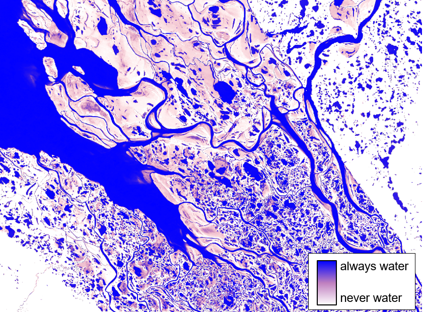
The Global Surface Water’s Occurrence map shows the fraction of time an observable Landsat pixel was water.
You can relatively quickly train and apply ML models using Google Earth Engine, although the learning curve may be a little steep if you haven’t used it before.
DeepWaterMap is a trained deep convolutional neural network that you can apply to Landsat/Sentinel multispectral imagery to create your own masks. You can also improve DeepWaterMap’s base model by adding more training data. Requires some knowledge of Tensorflow.
A recent development as of April 2023 is the release of the Segment Anything Model (SAM) from Meta Research which allows rapid segmentation of any image, including satellite imagery. The SAM model has an API in Python via segment-geospatial that could be used for rapid identification of water from various satellite imagery sources, e.g. Planet or Landsat.
How do I edit my mask?
As a mask is simply a single-band image, any pixel-based image editing software can be used for hand-editing (Photoshop, GIMP, MSPaint, etc.). However, there are a few issues with using these tools:
These softwares will generally not preserve georeferencing information of your source image. You will have to add it back to the edited image.
The softwares may have difficulty opening/editing a single-band image as opposed to the more standard RGB (3 band).
Filetypes are sometimes not compatible between Python-exported images and these softwares and will thus require extra attention.
I have found three effective ways to edit georeferenced masks. The one you choose depends on the quantity and quality of editing you need to achieve.
Edit your mask directly in QGIS.
Paint.NET is an image-editing software that preserves georeferencing information. It’s fairly basic and easy to use. If you have a significant amount of hand-editing to do, look into it.
Use image processing tools in RivGraph to edit your mask. There are morphological operators like
rivgraph.im_utils.dilate()andrivgraph.im_utils.erode(),rivgraph.im_utils.regionprops()for filtering objects based on their properties (areas, lengths, perimeters, etc.), andrivgraph.im_utils.largest_blobs()for keeping/removing the largest connected components in the mask. There is also arivgraph.im_utils.hand_clean()utility that allows you to draw polygons one-at-a-time and specify their pixel values. I usually find these tools sufficient for cleaning a mask, regardless of the amount of editing required.
Does my mask need to be georeferenced?
Most masks are already produced in a GIS context and are already geographically referenced. However, RivGraph does not require that your mask image be georeferenced (e.g. a GeoTIFF). If you provide a mask without any georeference information, RivGraph will assign it a “dummy” projection in order to proceed. This has no effect on the network extraction. However, it is strongly advised that you provide a georeferenced mask. There are three primary reasons for this:
The coordinate reference system (CRS) of your mask will be carried through all your analysis, meaning that shapefiles and GeoTIFFs you export using RivGraph will align perfectly with your mask. Additionally, your results will be easily importable into a GIS for further analysis or fusion with other geospatial data.
RivGraph computes morphologic metrics (length and width) using pixel coordinates. A georeferenced mask contains information about the units of the mask, and thus any metrics of physical distance will inherit these units. If your CRS is meters-based, your results will be in meters.
Some of RivGraph’s functionality under the hood requires some heuristic thresholds or parameters. While these were designed to be as CRS-agnostic as possible, these functions will undoubtedly perform better when pixels have known units. As an example, generating a mesh along a braided river corridor requires some parameters defining the size and smoothness of the mesh. Having a mask with physically-meaningful units makes this parameterization much simpler and more intuitive.
Warning
You should avoid degree-based CRSs (like EPSG:4326). This is because the length of a degree is not uniform, but varies with latitude. For example, at the equator, a degree of longitude is roughly 111 km. In Anchorage, Alaska, a degree of longitude is approximately 55 km. Effectively, degrees are meaningless units of physical measurements. A more prudent approach would be to first project your mask into a meters-based CRS (e.g. the appropriate UTM zone) before analysis with RivGraph.
Can my mask represent something that isn’t a river?
Perhaps you’d like to vectorize a road network or a vascular system. This is possible to do with RivGraph. However, you will not be able to instantiate the convenient delta or river classes as they are designed only for river channel networks. Instead, you will need to poke around the API to figure out which functions will work for you. A good starting point is to skeletonize your mask with rivgraph.mask_to_graph.skeletonize_mask() then run rivgraph.mask_to_graph.skel_to_graph() to convert the skeleton to a set of links and nodes. If you have an interesting non-river use-case, please send an email to j……..k@gmail.com and we can add it as an example.
What filetypes are supported for my mask?
Any gdal-readable filetype should be fine. GeoTIFF is most common and recommended if possible.